


Higher-Penetration Costs of Wind and Solar
They're Potentially Astronomical
Introduction
Although no wind or solar generator produces electricity all the time, some such intermittent source is always generating somewhere. Opponents of fossil-fuel generation therefore contend that it can be replaced by simply transmitting electricity from locations where intermittent sources are currently generating to those where they aren’t. Exactly how much such an approach would cost is a complex question, and Naptown Numbers is unable to answer it with any precision.
But by simplified estimates based on load, wind, and solar data from the Energy Reliability Council of Texas (“ERCOT”), a future post will provide reasons for believing that the cost would probably be prohibitive. As background for that post this one will explore a related issue: the tendency for electricity prices to rise as intermittent sources supply an increasing fraction of the electricity demand. To provide focus we will begin by describing how that tendency differs from its description in a recent What’s Up with That post.
The Pollock Limit
Written by prominent climate skeptic Christopher Monckton, the What’s Up with That post reported that a researcher named Douglas Pollock had elegantly proved a previously unrecognized mathematical relationship between two quantities. The first quantity was intermittent-source penetration: the average fraction of total electricity that intermittent sources generate. The second quantity was the capacity factor: the ratio that the average power actually produced by those sources bears to their nameplate capacity. According to Lord Monckton’s post, what Mr. Pollock had proved was that penetration by a given type of electricity source cannot in the absence of storage exceed that type’s capacity factor.
Now, commenters in the ensuing thread promptly showed that the purported proof was in reality nothing more than an exercise in mathematical question-begging. But Francis Menton of the Manhattan Contrarian seemed to suggest that Mr. Pollock’s proof could be salvaged by limiting it to the case of no “overbuilding.” “By overbuilding,” Mr. Menton wrote, “I mean building so many generators that when the wind and sun are at full strength the system produces more electricity than the demand, which electricity then has to be discarded or wasted.” As the discussion proceeds we will see that even with Mr. Menton’s limitation the relationship Mr. Pollock purportedly proved is invalid.
The Underlying Data
But first we will use the load and wind-power records depicted by Fig. 1 to show that what the capacity factor does seem at first blush to approximate is the penetration at which the marginal cost of increasing penetration starts to rise.

Fig. 1’s load curve represents the ERCOT load data from 2020 and 2021. The wind-power curve is those same years’ total output of 155 wind farms listed in ERCOT’s wind-power data as “operational” but not “new for 2022.” Since all of the quantitative results in this post and the next will be based on this one data set we should recognize at the outset that to some degree our results would be different if we had based them on data from a different location—or from a different time period, for that matter. We will nonetheless obtain a qualitative sense of how cost depends on penetration.
We should also recognize that in discussing penetration we’re tacitly assuming a single, isolated electricity market in which the entire load has perfect access to all the market’s electricity generation. In this sense ERCOT is convenient because for regulatory purposes its system was designed to be relatively isolated from other markets. But that isolation isn’t actually perfect. Within ERCOT, moreover, there are limits to how much of the power generated in one region can be transmitted to another. So we’re employing a simplified approximation of a more-complicated reality.
The data indicate that those 155 wind farms have a total nameplate capacity of 25,558 megawatts (“MW”), whereas their total output had an average value of 9,961 MW: those wind farms’ aggregate capacity factor was (9,961 ÷ 25,558 ≈) 39%. The ERCOT load’s average was 44,145 MW, making the penetration of our selected wind farms amount to (9,961 ÷ 44,145 ≈) 23%. As Fig.1 shows, the load always exceeded the selected wind farms’ aggregate output.

Fig. 2 simulates a greater wind-farm output by so scaling Fig. 1’s wind-power curve as to make its average equal the load’s. It thereby shows that with increased penetration the wind power would exceed the load at some times and fall short at others. Since without storage the excesses can’t be used to make up for the shortfalls the resultant penetration is 75% rather than 100%. Still, that 75% penetration exceeds the wind farms’ 39% capacity factor. So at least as explained in Lord Monckton’s original post Mr. Pollock’s limit isn’t valid.
Penetration as Function of Installed Capacity
But now let’s scale up the original output values only as much as we can without overbuilding: let’s so scale the wind farms’ output as at some point exactly to satisfy but at no point ever to exceed the demand. The penetration we find when we do that is 31%, i.e., less than the 39% capacity factor. So the data we’re using seem to bear out the Pollock limit as Mr. Menton revised it: the penetration can’t exceed the capacity factor without storage or overbuilding.

By applying a range of scale factors to the wind-power data we can also see that the data are not inconsistent with the position to which Lord Monckton eventually retreated: that it’s costly and wasteful for penetration to exceed the capacity factor. Specifically, Fig. 3 shows that the rate at which penetration increases in response to increased nameplate capacity begins to decay after penetration exceeds the capacity factor.

That effect stands out better in Fig. 4, which interprets the reciprocal of Fig. 3’s derivative as proportional to the marginal cost of increasing penetration. Specifically, Fig. 4 so scales that reciprocal as to make the result begin at the $38/MWh average of Lazard Ltd.’s high- and low-end estimates of the levelized cost of wind power.1 For given levels of existing wind-power penetration Fig. 4 thereby estimates the levelized cost of so increasing the wind-power penetration as over time to have wind generate an additional megawatt-hour of electricity.
Although Fig. 4 is a good qualitative illustration of diminishing penetration returns to increased wind-power capacity, we caution against placing too much reliance on its particular cost values. We based our calculations on Lazard Ltd.’s numbers because those values are widely quoted. But Lazard based its numbers on a capital-cost range of $1025–$1350/kW with an average of $1188/kW, whereas a study based on audited UK company reports found the range of recently installed onshore wind to be about $1180–$2600/kW with a trend line’s latest value being about $2100/kW. So it’s quite likely that Fig. 4 understates marginal penetration cost.
The choice of the thermal-variable-cost line’s values was similarly rather arbitrary. Those values are a range of combinations of Lazard’s levelized-cost estimates for peaker and combined-cycle gas-turbine power plants. Since an increasing portion of the thermal plants need to operate in a less-efficient, load-following mode as intermittents’ penetration increases, we’ve arbitrarily started the weighting at 80% combined-cycle and 20% peaker operation, with the peaker percentage increasing linearly with penetration toward 100%.
One result of those choices is that even at minimal penetration wind’s marginal cost exceeds the estimates we’ve made of thermal sources’ variable cost. Not only were those choices somewhat arbitrary but in real life they also vary considerably with location and time. So one can’t confidently infer what that relationship seems to imply: that the marginal cost of increasing wind-power penetration always exceeds the savings it would afford in thermal-power cost. But we may speculate that it often does.
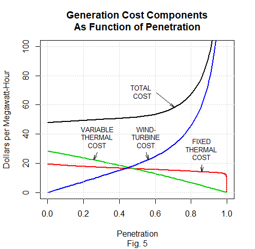
Fig. 5’s wind-turbine-cost curve is the integral of Fig. 4’s curve and thereby depicts cumulative wind-turbine cost as a function of penetration. Fig. 5’s total-cost curve represents the sum of that curve and its curves of the fossil-fueled back-up generators’ fixed and variable costs.
Note that the fixed-thermal-cost curve, representing back-up-generator costs such as debt payments and output-independent operation and maintenance, remains relatively flat until wind-power penetration has nearly reached 100%. That’s because the wind-power output’s minimum in the ERCOT record is so close to zero that for any plausible level of wind-turbine capacity there will always be some times when the thermal plants have to bear almost all the load.
For wind turbines alone to meet the demand despite that minimum their nameplate capacity would need to be nearly five hundred times the load’s average. So until the nameplate capacity reaches the astronomical level required to provide the final percent or so of penetration the back-up-capacity requirement decreases only slightly. And most of the decrease at low penetrations comes from our (again, somewhat arbitrary) assumption that if wind-power penetration is higher less of the gas-fired back-up capacity would consist of the more-expensive, combined-cycle plants.
Negative Correlation between Wind and Solar
To foreshadow the next post we will now show that the connection between the capacity factor and the penetration value at which electricity cost begins to rise is not as strong as it may have seemed so far. Specifically, by combining wind and solar we will increase that penetration value without increasing the capacity factor.
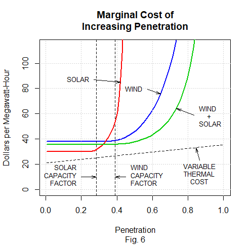
As Fig. 6 indicates, ERCOT’s solar-power data exhibit a capacity factor significantly lower than its wind-power data do. So it’s not surprising that the penetration at which marginal cost begins to climb is lower for solar than for wind. But it’s higher for the “wind + solar” curve even though the capacity factor of the 70:30 wind-to-solar weighting on which that curve is based is lower than that of wind alone.
That’s because the correlation between the wind and solar data is low—in fact, it’s significantly negative—and the sum of uncorrelated positive-valued functions tends to have a coefficient of variation lower than that of at least one of the addend functions. This means that for a given average value the peaks tend to be more modest than they’d be if the addends were more correlated, so the combined source’s output exceeds the load less frequently: less of the intermittent sources’ output is wasted.
Conclusion
So far we’ve seen the cost of 100% penetration remain prohibitive even though source diversity can somewhat reduce the cost penalty of increased penetration. The next post will show that geographical diversity could overcome that problem in theory but is unlikely to in practice.
April 13, 2023, update: That link is now broken, because Lazard removed the report whose data this post uses. That report has been replaced with a new report. We have not updated calculations in light of the replacement.