


Electricity-Generation Diversity
Beneficial but Probably Hard to Achieve
Introduction
Although no wind- or solar-powered generator produces electricity all the time, some such intermittent source is always generating somewhere. This post will therefore consider the possibility of eliminating fossil-fuel generation by simply transmitting intermittent-source electricity from locations where it’s currently being generated to those where it isn’t.
This post is a successor to a post in which we explored one of the reasons why electricity cost tends to increase with wind- and solar-power penetration: as penetration increases, more of such sources’ potential output goes to waste because it exceeds electricity demand more frequently. That post showed that this effect can be reduced to an extent by combining wind generation with solar. But it also showed that even with such source diversity the cost of increasing penetration eventually becomes prohibitive.
In this post we will see that the latter problem can be overcome in theory by geographical diversity, i.e., by drawing from sources so geographically distant from one another that their outputs aren’t very correlated. Exactly how much such an approach would cost is a complex question that we won’t attempt to answer with any precision. But we will make simplified estimates based on load, wind, and solar data from the Energy Reliability Council of Texas (“ERCOT”) that suggest the cost would be high.
Simulating Geographical Diversity
To simulate the low correlation that geographical distance might afford we differently time-translate copies of the ERCOT wind-power record we used in the previous post. (In this post we’ll concentrate on wind-power data only; although the previous post showed that mixing solar with wind can be beneficial, the inclusion of solar turns out not to confer much benefit on the combinations of de-correlated wind-farm outputs with which this post will deal.)

Figs. 7‑9 illustrate our approach to de-correlating those data. Fig. 7’s solid curve is the first ten days of the scaled-up wind-power curve we saw in the previous post’s Fig. 2. That curve is the sum of outputs generated by seven wind-farm groups into which we’ve divided the 155 wind farms. The dotted curves represent the running totals that result from adding respective group outputs.
Now, each group’s output differs from the others’. Even their correlations are low in some cases. But the average correlation between a single wind farm and the other 154 is 0.67, so on average the groups’ outputs reinforce one other’s peaks and troughs, making their sum highly volatile.
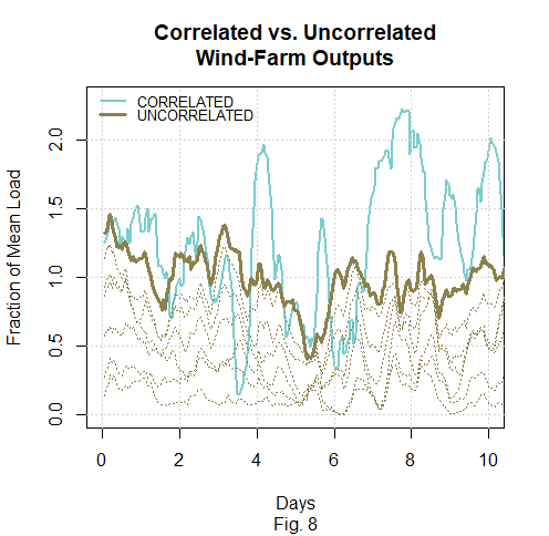
Now let’s time-shift each output from all the others to simulate the result of having geographically separated those wind-farm groups enough that they’re no longer very correlated. When we do that we find that some resultant correlations are positive and some are negative but that their magnitudes are all less than 0.1. As Fig 8 shows, the peaks and troughs in the groups’ outputs therefore tend not to reinforce one other. The result is that the sum’s peaks and troughs are less pronounced.
De-Correlation and Overbuilding
Fig. 9 below illustrates how such a variance reduction could affect the penetration value at which overbuilding begins. Its wider-variance wind-power curve represents our original, pre-de-correlation sum of 155 Texas wind farms’ outputs scaled up to just short of overbuilding. As we previously observed, the resultant penetration is about 31%.
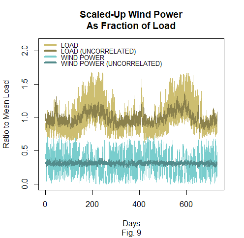
Its lower-variance wind-power curve results from the type of de-correlation by time-shifting that Figs. 7 and 8 illustrated. But instead of de-correlating among only seven groups we’ve exaggerated the effect by time-shifting each of the 155 individual wind-farm outputs from every other one. We haven’t thereby changed the average output or the 39% capacity factor our previous post mentioned. But de-correlation has so decreased the coefficient of variation that the sum comes nowhere near to overbuilding. The uncorrelated wind farms’ aggregate output could be scaled up to 51% penetration without overbuilding, not just to the illustrated 31%. Contrary to one reported contention, therefore, there’s no reason in theory why wind-power penetration couldn’t exceed the capacity factor without overbuilding.
To an extent geographical diversity among load components, too, would reduce correlation; sometimes electricity demand decreases in one region when it increases in another. So we’ve time-shifted the records of the eight regions among which ERCOT divides its load, and Fig. 9’s narrower-variance load curve depicts the resultant sum. The consequent reduction in the aggregate load’s coefficient of variation would increase the overbuilding threshold from 51% penetration to 65%.
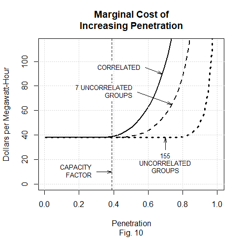
As Fig. 10 shows, in fact, penetration can be increased significantly beyond that value before overbuilding has much of an effect. Fig. 10’s solid curve is the same as Fig. 4’s from the previous post: based on that post’s wind-turbine-cost assumptions, it results from the 155 original, relatively correlated wind-farm outputs and the eight original, highly correlated regional loads. The dashed curve results from de-correlating seven wind-farm groups as Figs. 7 and 8 illustrated and replacing the load with the sum of two de-correlated load groups. The dotted curve results from 155 de-correlated wind-farm outputs and eight de-correlated load groups.
The dotted curve shows that—if the simulated de-correlation could be achieved—penetration could increase to 80% before the marginal cost would begin to increase significantly. As we will now see, in fact, there’s no reason in theory why 100% penetration could not be achieved.
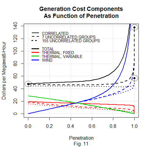
Fig. 11’s solid curves replicate those of the previous post’s Fig. 5, which represented the cost-component values obtained by simply scaling up the ERCOT data. The dashed and dotted curves represent corresponding values based on respective sets of Fig. 10’s de-correlation assumptions.
The circled points on Fig. 11’s right are the ends of the total-representing black dashed and dotted curves. They show that under those curves’ assumptions the costs of 100% penetration aren’t the astronomical values in which more-correlated sources result. Indeed, comparison of the lower circled dot on the right with its counterpart on the left reveals that wind-only generation in the 155-region simulation isn’t much more expensive than fossil-fuel-only generation.
The differences among those total-cost curves reflect differences among wind-turbine costs and among fixed thermal costs. The reason why the dashed and dotted fixed-thermal-cost curves decline more significantly at low penetrations than the solid one does is that de-correlating the wind-power sources reduces the wind-power troughs’ depths and thereby makes wind-power penetration more effective at reducing the need for fossil-fueled back-up capacity. And the penetrations at which the wind-turbine-curve slopes begin to increase are greater for the dashed and dotted versions because that de-correlation reduces the wind-power peaks and thereby the fraction of available wind power that goes to waste.
Again, the cost of all-wind-power generation in the 155-group simulation barely exceeds that of all-fossil-fueled generation. And by plausible changes in some of the parameter values we could easily have made it lower still. So Fig. 11 seems to support the proposition that enough geographical diversity could solve wind power’s intermittency problem without much added cost.
Correlation and Distance
But there are reasons to question that proposition. So far, for example, the real world has not provided much evidence that high penetrations of intermittent-source generation can be less expensive than all-fossil-fueled generation; real-world electricity prices tend to be higher in higher-penetration locales. As we will now see, moreover, the relationship between correlation and distance in the ERCOT data suggests that as a practical matter the benefit of geographical diversity couldn’t much exceed what our seven-region simulation exhibits.
Even before we de-correlated their outputs the wind-power correlations between Panhandle and Gulf Coast wind farms in the ERCOT data were just about zero . As we stated before, though, the average correlation between any individual wind farm and the 154 others was 0.67. That’s because nearly three-quarters of the wind-power generation was concentrated in West Texas and the Panhandle.
Those facts tell us two things. First, intermittent sources can’t always be sited conveniently; otherwise, wind-farm developers wouldn’t have sited half of them in West Texas, where relatively little of the generated electricity is consumed. Second, obtaining the simulated degree of de-correlation in real life can require a lot of distance; the distance between Amarillo in the Panhandle and Corpus Christi on the coast is about 700 miles. Even reducing the distance to the 500 miles between Amarillo and the southern region’s San Antonio increases the Panhandle region’s output correlation from 0.02 with the coastal region to 0.17 with the southern region.
So let’s say for the sake of discussion that regions’ centers would have to be at least 500 miles apart to be as uncorrelated as they are in our simulations. Then the wind farms of the 155 uncorrelated regions represented by Fig. 11’s dotted curves would have to be spread somewhat evenly over an area that’s around 7000 miles in diameter. That’s obviously impractical. From here on out we will therefore ignore the 155-region simulation.
But it isn’t completely inconceivable for the wind farms to be spread over the 1500-mile-diameter area that seven uncorrelated regions would occupy. (Envision a central 500-mile-diameter region abutting six surrounding ones.) Still, such an area centered on Indianapolis would extend from the Atlantic Coast to central Nebraska and from the Gulf Coast well into Ontario. And a greater area would be needed if the wind farms couldn’t be spread out uniformly but instead were lumped together in more wind-favorable but load-distant sites as they tend to be in Texas.
As Robert Bryce reports, moreover, the permitting hurdles typically encountered by interstate transmission-line projects entitle us to question whether enough interconnection capacity could be added before well into the next century. So even our seven-uncorrelated-region simulation seems optimistic—and that simulation’s cost of 100% penetration is nearly three times the cost of thermal-only generation. We should therefore be skeptical of arguments that geographical diversity alone can enable us to eliminate thermal generation—at least at a reasonable cost.
Enter “Social Cost”
But wind power’s cost can be made to appear less unattractive by imposing a “carbon” tax on fossil-fueled generation, purportedly to capture in the price signal carbon-dioxide emission’s otherwise-omitted “social cost.” If burning a million BTUs’ worth of natural gas produces 52.91 kilograms of carbon dioxide and the heat rate of our fossil-fueled generation ranges from 7000 to 8900 BTU/kWh as wind-power penetration increases from 0% to 100%, then adding $19–$24/MWh to our $28–$36/MWh variable-cost assumption would internalize the $51 contended by the Biden administration to be the social cost of emitting a metric ton of carbon dioxide.
Now, that social-cost estimate is probably exaggerated. A recent study concluded, for example, that the social cost is unlikely to be much more than a tenth of the Biden-administration value. And a reply to a critique of that study applied the critique’s recommendations to arrive at a median value in 2050 of $3.39/t with a 33.4 percent probability that the optimal carbon tax would actually be negative. But we’ll stick with the $51/t level in Fig.12 below to illustrate imposing a tax in the seven-uncorrelated-region scenario.
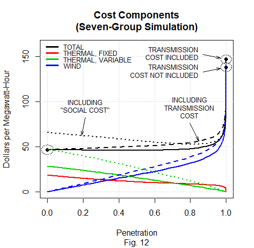
Fig. 12’s solid-line curves replicate Fig. 11’s dashed-line ones, while its dotted lines result from adding the carbon tax to the thermal sources’ variable cost. Comparison of the circled dot on the left with the lower one on the right reveals that not even a $51/t rate would make it attractive to eliminate fossil-fueled generation completely.
Transmission Lines
Since fossil-fuel opponents contend that fossil fuels impose social costs not captured by the price mechanism, we should mention that wind turbines impose costs like grid instability and wildlife loss that we haven’t captured here. As a sort of placeholder for such costs we’ll now add numbers for another hard-to-evaluate cost: that of the added transmission-line capacity that geographical diversity requires. Texas has already spent billions to add the transmission lines its wind power requires, yet its wind-farm outputs’ correlations still average 0.67. So achieving the correlation reductions we’ve simulated would cost much more.
How much more is hard to estimate; the costs of high-voltage transmission lines seem to vary widely. For the five that Mr. Bryce reported, for example, they ranged from $0.74 to $7.65 per kilowatt-mile, with an average of $2.59. But to make a rough guess we’ll use those examples’ $1.14/kW/mi. median value.
The average distance from a location in a 1500-mile-diameter region to a load at its center is about 530 miles, so even if the ratio of required transmission capacity to average load is only 1.3 the capital expenditure would be $789/kW (= 1.3 × $1.14/kW/mi × 530 mi.). Financing that expenditure at rates the same as Lazard uses to estimate generation-capacity expense (60% debt at 8% and 40% equity at 12%) would add $8.64/MWh to the 100%-penetration wind-turbine cost. Fig. 12’s dashed curves represent the result of making that addition.
The dashed black curve’s monotonic increase tells us that under these assumptions the thermal-generation expense saved by adding wind-power capacity wouldn’t justify the wind turbines’ cost even at low penetrations. Of course, carbon-tax rates can be so set as to make it appear that they would. But a comparison of the circled dot on the left with the upper one on the right suggests that the rate would have to be very high indeed to make complete fossil-fuel elimination appear attractive.
Note also that in this as in other instances we have probably biased our estimate in wind’s favor. Our estimate would have been three times the $8.64/MWh value we arrived at above if instead of the median transmission-line cost we had used the average and instead of a 1.3 max-to-mean ratio we had used the ERCOT load’s 1.68. And it would have been higher still if we had included the cost of increased transmission-line operation and maintenance.
Battery Storage
As we stated above, adding solar to the mix turns out not to help much once wind power is uncorrelated enough, at least if our ERCOT data are representative. But what about battery storage? True, we found in a previous post that providing enough batteries to make wind reliable is almost certainly too expensive. But that conclusion wasn’t based on uncorrelated sources. So here we will base the assessment on our seven-uncorrelated-region simulation.
To that end we assume that financing enough batteries to store an hour’s worth of average load adds $2.22/MWh to the cost of generating electricity. We obtained this value by taking the yearly payment for that much storage to be $19,435 per megawatt of average load. That yearly-payment cost was in turn based on an assumed battery cost of $153/kWh financed over twenty years at the 11.2% (20% debt at 8% and 80% equity at 12%) rate that Lazard uses for that purpose.
Although that financing rate may seem high, it’s not much higher than the rates on which Lazard’s fossil-plant and wind-turbine numbers were based, and there are reasons for believing that the resultant payment estimate is conservative. Specifically, the twenty-year term seems generous for batteries, and the $153/kW price we assumed is much lower than, say, those in the $400 to $600/kWh range recently reported for Tesla Megapacks. Moreover, that $153/kWh results from reducing Lazard’s $172/kWh battery-cost estimate by its stated inverter cost on the theory that longer-term storage may not need to be capable of as much power as is required by the intra-day cycling Lazard seems to have assumed.
The estimates we made above are obviously debatable. But they could be changed quite a bit without disturbing the qualitative conclusion we’ll draw from Fig. 13 below: that up to a point the addition of storage can reduce the cost of completely eliminating fossil-fueled back-up generation.
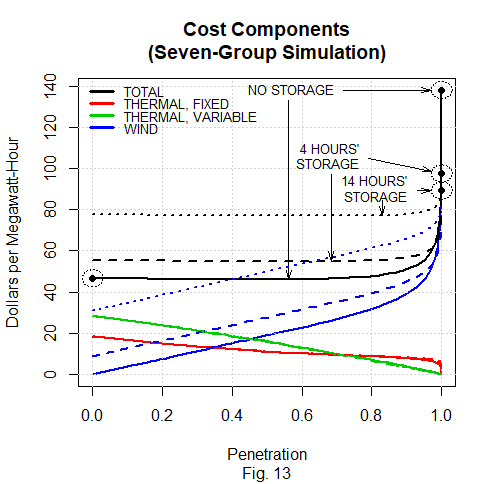
That plot’s dashed and dotted curves result from including the respective costs of four hours’ and fourteen hours’ worth of storage in our seven-region simulation’s wind-turbine component. For the sake of simplicity we’ve ignored charge and discharge losses, so we’ve again biased the analysis in wind’s favor, this time by overstating the savings from battery use. We’ll ignore those curves’ left-hand portions because they’re actually unrealistic; they include the battery cost even at zero penetration, when there’s no wind-turbine output for the batteries to store. Their right-hand portions are what we’re interested in.
For penetrations much below 100% those portions tell us that overall cost rises with storage capacity. But the circled dots at their right ends tell us that by 100% penetration the cost order has reversed: the greater the storage, the lower the cost. The reason why more storage results in lower cost at 100% penetration is that overbuilding, which is what battery storage mitigates, occurs disproportionately in obtaining that last bit of penetration.
What Fig. 13 doesn’t show is that beyond about fourteen hours’ worth the cost of more storage exceeds the wind-turbine cost thereby saved: under our assumptions fourteen hours is approximately the optimal storage capacity. And comparison of the circled dot on the left with the lowest one on the right tells us that even when the storage level is optimal all-wind generation is nearly twice as expensive as all-fossil-fuel.
To tilt that comparison in wind’s favor would require imposing a carbon tax of more than $108 per metric ton of carbon dioxide: over twice the Biden administration’s probably exaggerated $51/t social-cost estimate. If the transmission-line cost from Fig. 12 is included that tax would have to be over $140/t.
Conclusion
We have seen that it is theoretically possible to obtain reliable electricity from intermittent sources by exploiting the low correlation that geographical diversity can provide. As we said at the outset, we don’t profess to have determined with anything like precision what that approach’s cost would be. But calculations we probably biased in wind’s favor showed it’s likely to be exorbitant even though we ignored drawbacks such as increased instability risk and the reliability penalties of transmitting more power over longer distances.
So we would be wise to require compelling evidence before we perpetuate subsidies and regulatory mandates that prop intermittent generation up on the theory that geographical diversity will eventually make intermittent-source electricity generation cost-effective.