Cold Stove Lids and Convolution I

The Math Error at the Heart of an “Irreducibly Simple Climate Model”

Introduction

This post and the next two will be directed to a fundamental error at the heart of a 2015 Monckton et al. paper, “Why Models Run Hot: Results from an Irreducibly Simple Climate Model.” Although that paper generated a certain amount of buzz when it was first published, our impression is that it has largely faded into well-deserved obscurity. So the reader is warned that despite its climate connection the following discussion is unlikely to have any real policy implications; it may best be looked upon as merely a review of some college math.

Still, this post was prompted by an interview last month in which lead author Christopher Monckton claimed a causal link between that paper and the first Trump administration’s withdrawal from the Paris Climate Agreement. So we can’t completely rule out the possibility that the paper may yet have an impact.

And that would be unfortunate, because it has numerous flaws, such as a misinterpretation of the equilibrium relationship among loop gain, open-loop gain, and closed-loop gain that led the authors to claim that climate models “used the wrong equation.” But the flaw we’ll concentrate on in these posts will be its Equation 1 tenet that the output with which a linear system will respond to a given input can usefully be approximated simply as numerically equal to the product of that input and the output the system would have responded with if the input had instead been a unit step function.

To provide background this post will employ a simple first-order model and simple pulse stimulus to review convolution, which is a mathematical operation often used in calculating a linear time-invariant system’s response to a given input. Using that same model and stimulus, the next post will show how the Monckton et al. estimate can be too wide of the mark to be of much use. And by using a more history-based stimulus function and a more climate-like model the third post will demonstrate that with respect to the experience that Lord Monckton has claimed the climate is what we’ll call a “cold stove lid.”

The Monckton et al. “Model”

Monckton et al. refer to their Equation 1 as a climate “model.” That viewpoint is defensible, but in this post we’ll view their equation instead as a formula for estimating the output of someone else’s model. The model whose output they used their Equation 1 to estimate is the one that generated the step response depicted in Gerard Roe’s “Feedbacks, Timescales, and Seeing Red.” Monckton et al. based their estimates on that step response itself rather than on the model equations that Dr. Roe used to generate it. Although the Equation 1 approach is erroneous, a time-invariant linear model’s output can indeed be calculated from its step response and the applied stimulus. Before we describe how such a calculation is done we’ll consider certain distinguishing linear-systems features.

Linear Systems

It’s true, of course, that the climate is far from a linear system. But a nonlinear system’s behavior can often be reasonably estimated by linear models if consideration is limited to a narrow range of operation. Such models typically consist of differential equations that define the relationship between the system’s input or stimulus x and its output or response y. In the Roe paper the output is the difference between average earth temperature and some reference value, while the input is what’s called climate “forcing.”

Various refinements sometimes get tacked onto the Intergovernmental Panel on Climate Change (“IPCC”) definition of forcing, which is that it’s “the change in the net, downward minus upward, radiative flux (expressed in Watts per square metre; W m^-2) at the tropopause or top of atmosphere due to a change in an external driver of climate change, such as, for example, a change in the concentration of carbon dioxide (CO₂) or the output of the Sun.” Moreover, the IPCC definition might have made it clearer that the forcing associated with, say, a carbon-dioxide-concentration change is looked upon as remaining so long as the resultant concentration does, even after the temperature response to that change has redressed the initial radiative imbalance the change initially caused. But those details need not detain us, because forcing’s precise definition won’t be important in this discussion.

Our focus will simply be the model equations that define relationships between forcing, however defined, and the resultant temperature response. Or, rather, it will be the responses that those model equations generate; the Roe paper whose model output Monckton et al. attempted to approximate didn’t provide its system equations, which in any event would have been more complex than our description of basic linear-systems properties will require.

So for explanatory purposes we’ll initially just assume the extremely simple model defined by the following equation:

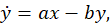
where the dot over the y denotes time differentiation and a and b are constant coefficients of proportionality. This equation says that the rate at which the output y changes equals the difference between quantities respectively proportional to the input and the output.

A climate-context interpretation, for example, could be that the earth temperature’s rate of change is reduced from a forcing-proportional term’s value by a quantity proportional to the temperature itself. As the temperature output y increases, in other words, the outgoing radiation does, too, and thereby limits the temperature increase that radiation absorption would otherwise cause. (Again, the temperature we’re referring to in this context isn’t absolute temperature but rather the difference between the absolute temperature and the temperature reference that’s being used for linearization.)

Unknown System Equations

If the input x is known as a function of time then the output y can readily be calculated from its initial value and the model equation above by using a conventional technique such as the numerical one we described in “Mars Flyby I.” As we pointed out above, though, the model equation isn’t necessarily known in the situation with which the Monckton et al. paper concerns itself. What is known instead is the system’s response to a unit-step-function stimulus, i.e., to a stimulus that equals zero at all times before time t = 0 and equals one at all times thereafter.

As we stated above, Monckton et al.’s Equation 1 therefore purports to base approximation of a system’s output on what its output would have been if the stimulus had been a step function. As background for our next post’s demonstration that it goes about this in the wrong way this post will describe the correct approach. And that approach is based on “superposition.”

Superposition

When we say that our simple demonstration system is linear we mean that in its system equation neither the input, nor the output, nor any time derivative of those quantities is squared or otherwise raised to a non-unity power. A result of this linearity is superposition: a linear system’s response to an input that can be expressed as a sum of constituent inputs equals the sum of the individual responses to those constituent inputs. If those individual responses are known the response can therefore be calculated as that sum; the system equations themselves need not be known.

The plots above illustrate this feature. The stimulus curve at the bottom left is the sum of the two stimulus curves above it, to which the top two curves on the right are our demonstration system’s corresponding responses if its coefficient values are a = b = 1. (The present discussion doesn’t depend on what the input and output dimensions are, so we’ve dispensed with them.) Since the system is linear the composite stimulus’s response shown by the bottom right plot equals the sum of the individual responses to the constituent stimuli.

As a solution tool superposition is particularly powerful when the linear system in question is time-invariant, as the Roe model presumably is. Recall in this connection the assumption that our demonstration model’s coefficients a and b are constants. Linearity doesn’t really require constant coefficients; so long as a and b are independent of the stimulus and response the demonstration system would be linear even if those coefficients were time-dependent. But a benefit of time invariance is that time translation doesn’t change the system’s response.

Since Fig. 1’s second-row stimulus is merely a time translation of its first-row stimulus, for instance, time invariance tells us that the second-row response will similarly be just a time translation of the first-row stimulus. So we wouldn’t need to know the second stimulus’s response a priori in order to calculate the third-row response; we could infer it from the first response.

Moreover, this result doesn’t require that the second-row stimulus exactly equal a time translation of the first-row stimulus. Linearity enables us to infer the second-row response from the first-row response even if the second-row stimulus is just proportional to such a time translation: the second-row response would simply be the time translation of the first-row response scaled by the two stimuli’s amplitude ratio.

Convolution

Fig. 2 illustrates how a given arbitrary stimulus can be approximated by summing scaled and time-translated replicas of a base stimulus function.

Again, we can approximate a time-invariant linear system’s response to the given composite stimulus by summing time-translated and scaled replicas of the basis stimulus’s response. Moreover, although such an approach’s result is merely an estimate, it approaches exactitude as the pulse duration approaches zero. The plot below illustrates taking the thereby-approached limit of the pulse response.

The duration and amplitude, and therefore the time integral, of the dashed red pulse are all unity. The solid red curve represents the example system’s response to that pulse. So the response to any stimulus that can be approximated as a sum of translated and weighted replicas of that dashed red pulse can be estimated as the sum of correspondingly translated and weighted replicas of that solid red response.

But better approximations would tend to result from shorter-duration pulses such as the green pulse. The green pulse’s duration is only half the red pulse’s, but it has the same, unity time-integral value because it has twice the red pulse’s amplitude. The solid green curve shows that for our particular system the response to the higher-amplitude but shorter-duration pulse initially climbs faster but starts to decay sooner, so the two responses approximate one another after the stimulus pulses have passed.

If we continue to reduce the pulse duration in this manner the limit as that duration approaches zero is the function represented by the solid black curve. That function is sometimes referred to as the system’s “impulse response,” or its response to the Dirac delta function. (The Dirac delta function of time t is defined as having a function value of zero for non-zero time values but having a time integral of unity over any interval that brackets time t = 0.) In the limit the response y to an arbitrary stimulus x therefore equals the sum of an infinite number of time-translated infinitesimal-magnitude replicas of that impulse response scaled by corresponding values of the stimulus x.

Now, the manner in which we’ve just used impulse response suggests that its units would be those of the system response. But we’ll now treat its units as being those of system gain—i.e., those of the ratio of output to input—per unit time and give it the symbol h(t) so that we can express the just-described infinite summation as follows:

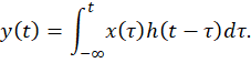
The operation performed by that integral is known as convolution and is a standard approach to calculating linear-system outputs.

But the type of convolution we’ve just described requires knowing the impulse response h(t), whereas what’s known in the case illustrated by the Monckton et al. paper is instead the system’s response to a step function. For mathematical convenience we’ll sometimes use the term step response to refer not to that response itself but rather to the function that’s numerically equal to it but has units of system gain.

Whereas the system’s impulse response h(t) increases instantaneously to an initial value from which it thereafter decays exponentially to zero, its step response u(t) increases gradually from zero and asymptotically approaches an equilibrium value, which our particular coefficient choice has caused to be unity.

Now, the impulse response can readily be inferred by differentiation from the step response. But the step response can also be used directly in the convolution integral if the stimulus is replaced with its time derivative.

To see why this is so consider the above-illustrated stimulus function. Like Fig. 1’s top-left function it consists of a single, unit-duration pulse. That pulse is constant throughout its domain except at times t = 1 and t = 2, where respective +1 and –1 changes occur. So the pulse initially behaves like a unit step delayed from t = 0 to t = 1, and the plot displays the step-response curve so translated as to begin at t = 1 instead of t = 0.

The stimulus pulse’s return to zero at t = 2 is equivalent to subtracting a further-delayed step from that original step. The plot therefore includes a corresponding further-delayed step-response curve. Since the second stimulus step is subtracted, so is the second step response: the shaded area between the two step responses represents those step responses’ difference, and the bold curve, equaling that shaded area’s vertical extent, is the overall pulse response we saw in Fig. 1’s top-right plot.

If a stimulus can be approximated by a sequence of increasingly delayed pulses, therefore, a linear time-invariant system’s response to it can be approximated by the sum of a sequence of correspondingly delayed step responses weighted by the amplitude changes between successive pulses. And the resultant estimate approaches exactitude as the pulse duration approaches zero:

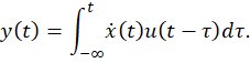
That is, the response can be expressed not only as the convolution of the stimulus with the system’s impulse response but also as the convolution of the stimulus’s time derivative with the system’s step response.

Stay Tuned . . .

In this post we’ve reviewed the correct way of calculating a system’s output from its input and step response. In the next one we’ll compare the model output thus calculated with the estimate that Monckton et al.’s approach would produce.