
Cold Stove Lids and Convolution III
The Math Error at the Heart of an “Irreducibly Simple Climate Model”
Introduction
As this post will, our two previous posts dealt with the estimation formula set forth in Equation 1 of Monckton et al.’s “Why Models Run Hot: Results from an Irreducibly Simple Climate Model.” Those two posts demonstrated that as a theoretical matter the discrepancy between a model’s actual response to a given stimulus and the estimate thereof produced by the Monckton et al. formula could be too great for the estimate to be of much use.
But lead author Christopher Monckton has claimed that the discrepancy isn’t so great if we limit consideration to the climate context. And it’s true that for the sake of simplicity the stimulus and step-response functions used in the previous post’s demonstration were less typical of the climate than they might have been. So this post will show that the discrepancy can be too great even in a climate context.
Epidemiology
Lord Monckton’s argument for accuracy in the climate context was based on an epidemiological experience he claimed:
As it happens, I had first come across the problem of stimuli occurring not instantaneously but over a term of years when studying the epidemiology of HIV transmission. My then model, adopted by some hospitals in the national health service, overcame the problem by the use of matrix addition, but sensitivity tests showed that assuming a single stimulus all at once produced very little difference compared with the time-smeared stimulus, merely displacing the response by a few years. Similar considerations apply to the climate.
Leaving aside whether Lord Monckton truly understood the issue, we must admit that climate forcing doesn’t exhibit the types of sudden changes that the pulse stimuli in our previous post did. Furthermore, the step response of the simple first-order demonstration model we used there tended to rise more slowly at first than the step responses Monckton et al. used, and it tended thereafter to approach its equilibrium value more quickly.
But what we’ll find by using functions that are more climate-typical is that if Lord Monckton’s epidemiological experience was indeed the authors’ reason for adopting as mathematically incoherent an approach as they did they failed to heed Mark Twain’s following admonition:
We should be careful to get out of an experience only the wisdom that is in it and stop there lest we be like the cat that sits down on a hot stove lid. She will never sit down on a hot stove lid again and that is well but also she will never sit down on a cold one anymore.
Climate-Like Stimulus and Step Response
The stimulus we’ll use in order to determine whether “similar considerations” really do “apply to the climate” is the following more-gradual forcing record, which we’ve inferred from the historical CO2-concentration-equivalent values that the Coupled Model Interconnection Project (“CMIP”) was recommending when Monckton et al. wrote their paper.
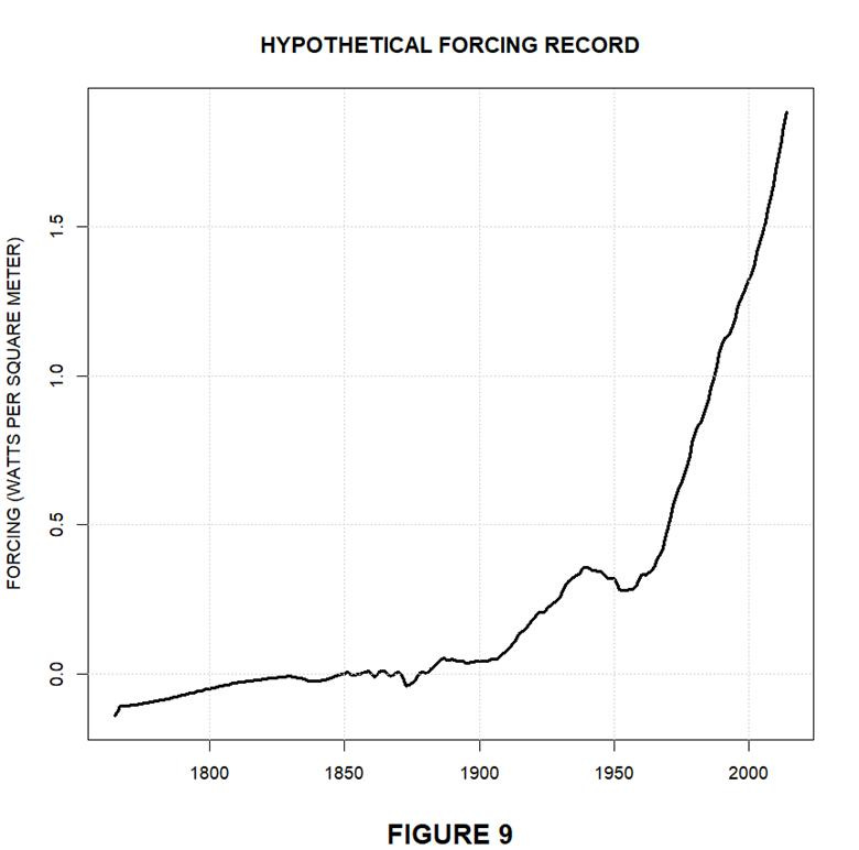
That stimulus function doesn’t exhibit the sudden large changes that our previous one did. Being a CMIP recommendation, moreover, it’s obviously the type of stimulus function on which climate models are likely to operate.
Basically, the step-response function we’ll use is based on the fourth row of Monckton et al.’s Table 2, whose entries in turn were based on a plot in Gerard Roe’s “Feedbacks, Timescales, and Seeing Red.” However, those entries were apparently eyeballed, because the curve they produce would be more jagged than Dr. Roe’s. Anyway, their time resolution would be too coarse.
So we’ll generate smoother, higher-resolution step responses by using a feedback model that’s similar to the one diagrammed by the previous post’s Fig. 6 but that employs a different network within that diagram’s dashed rectangle.
The replacement network will exhibit the following third-order relationship between its output y and its block input z ≡ x + fy:

subject to the constraint that p0 ÷ q0 = λ0 so that the overall system’s equilibrium open-and closed-loop gains are respectively forced to be λ0 and λ∞ = λ0 / (1 – λ0f).
Our choice of the third order was largely arbitrary, the thought being that it would provide enough free parameters for reasonable curve fitting. Note that despite the higher order we’ve still not assumed any storage in the outer feedback path. In truth, the principal reason for that choice was just to spare ourselves complexity. However, our guess is that on the time scales involved here many searchers would find it a reasonable estimate.
Anyway, we so chose the p’s and q’s as to produce a step response roughly similar to the one that the middle, mean-value curve in Monckton et al.’s Fig. 4 below implies.
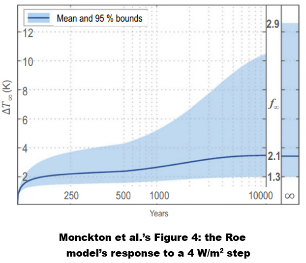
Monckton et al. adapted their Fig. 4 from the Roe paper’s Fig. 6, which graphed its model’s response to a 4 W/m2 forcing step. (Note that the apparent convexity in the middle of the curve is an artifact of the time scale’s nonlinearity; in all likelihood the function is entirely concave.) Presumably by assuming their paper’s 0.3125 K·m2/W value of open-loop gain λ0 and eyeballing the Roe curve’s value for t → ∞ they inferred the f = 2.1 W/m2/K feedback-coefficient value they labeled the curve with.
And they apparently calculated the so-called transience-fraction values rt in their Table 2’s fourth row by taking the ratios that the curve’s intermediate values, which they presumably also eyeballed, bore to its final value. The step-response values represented by the dots in the following plot’s dashed red curve are products of those transience-fraction values and the equilibrium closed-loop-gain λ∞ value implied by the λ0 = 0.3125 K·m2/W and f = 2.1 W/m2/K values that Monckton et al. used.

We used those dots to obtain the p’s and q’s in our previously stated relationship between the forward-block input and output z and y. (That forward-block relationship can also be thought of as the open-loop relationship between the whole-system input and output x and y.) Specifically, we so adjusted those coefficients that when we close the loop with the inferred f = 2.1 W/m2/K feedback-coefficient value the resultant system’s step response is Fig. 10’s solid-green-curve approximation of the red curve.
The Roe plot’s shaded area represents the range of responses that result from a corresponding range of feedback coefficients. By using different feedback-coefficient values f with our common open-loop equation we similarly obtained a family of different step-response curves. For a reason that will become apparent, the family member we’ll multiply by the Fig. 9 stimulus function to illustrate Monckton et al.’s output-estimate approach is the result of using f = 1.6 W/m2/K as our feedback-coefficient value.
Applying the Monckton et Al. Approach
As the previous post pointed out, one of the failings of the Monckton et al. approach is that its output depends on the user’s choice of time origin. To use it, that is, we have to make a choice that’s essentially arbitrary; Monckton et al. are silent as to precisely what that choice should be in any given case.
The choice we’ve made is to place the origin at the year 1850: that will be the point in the record that we align with the step response’s year zero. We made that choice because the authors take 1850 as the start of the industrial era and purport to draw conclusions from the 0.8° temperature increase they claim had occurred between that year and the year 2014.

The above plot’s solid red and green curves depict the resultant estimated and actual model outputs. Obviously, the sign and magnitude of the difference between the estimated and actual values change over the years, but Monckton et al.’s estimate of the overall change would be 50% greater than the true value. And a 50% discrepancy seems significant.
But let’s base our assessment of that discrepancy’s significance on the purpose to which the model would be put: determining how much feedback there is in the climate system and thereby how great a temperature change a given increase in carbon-dioxide concentration will ultimately cause. Monckton et al. would have us base such a determination on using models like Dr. Roe’s to match the 0.8°C temperature change purportedly observed since 1850. And although we doubt that there are many serious researchers on either side of the climate debate who would think much of such an approach we’ll set our reservations aside and adopt it here.
Fig. 11’s red curve shows that if in doing so we used Monckton et al.’s Equation 1 to calculate the models’ outputs we would arrive at f = 1.6 W/m2/K as the best-match feedback-coefficient value. Furthermore, multiplying the thereby-implied equilibrium closed-loop gain λ∞ = λ0 / (1 – λ0f) = 0.3125 K·m2/W ÷ (1 – 0.3125 K·m2/W × 1.6 W/m2/K) = 0.625 K·m2/W by the 3.708 W/m2 value that the authors give for the forcing associated with a doubling of the carbon-dioxide concentration implies that the so-called equilibrium climate sensitivity (“ECS”)—i.e., the temperature change in which doubling the carbon-dioxide concentration would eventually result—would be about 2.3°.
But that’s all based on the Monckton et al. estimate. As Fig. 11’s green dashed curve indicates, the feedback value we’d arrive at by using the model’s actual output would be more like 2.7 W/m2/K—which implies an ECS value closer to 7.4°. The ECS value implied by the model’s actual output, that is, would be more than three times what Monckton et al.’s estimate of that output would imply.
Few honest observers would dismiss this as “very little difference.” So climate appears to be Lord Monckton’s cold stove lid: whatever wisdom his epidemiological experience may have contained doesn’t extend to the climate.
True, Fig. 11 is based on a number of assumptions, such as where the time origin should be placed. We could no doubt have made assumptions under which Monckton et al.’s Equation 1 would give better estimates. But for any given set of assumptions the only way of knowing whether Monckton et al. would get close is to perform the actual convolution or other calculation of what the model’s real output is. And once the exact model output is thereby known there’s no point in using Equation 1 to calculate a mere estimate.
Conclusion
Again, the foregoing discussion should probably be looked upon as largely academic; at least prior to the Tom Nelson Podcast interview that we mentioned in the first post the Monckton et al. paper seemed to have sunk into obscurity. Even in that interview, moreover, the real subject was not the 2015 paper but rather the authors’ successor, forgotten-sunshine theory (which we discussed three years ago in “The Power of Obscure Language”).
Still, Lord Monckton claims that the 2015 paper was downloaded more often by a factor of twelve than any other paper published by the journal it appeared in. According to him, moreover, it caused officials in the first Trump administration to open communications with him that he at least strongly implied led ultimately to U.S. withdrawal from the Paris Climate Agreement. (“I was asked to send a one-page brief to Donald Trump, which I sent, and within one week he had pulled America out of the Paris Climate Agreement.”) He further claimed that the paper was a cause of at least one co-author’s being “knocked out” of his institution.
Independently of how true such claims may be, the fact remains that Lord Monckton seems remarkably able to attract a following for even the most-preposterous theories. And since even a critical reviewer called its mathematical derivation “impeccable” there may still be some value in having the public record include this analysis of its central error.