The Power of Obscure Language
You Can Fool Some of the People All of the Time
Introduction
Although climate models employ well-understood physics, there are some phenomena, such as clouds and thunderstorms, that remain poorly understood and in any event occur at spatial resolutions too fine for modelers’ still-limited computational capacity to handle. This forces modelers to supplement established physics with guesses (euphemistically called “parameterizations”), and many of us believe that such guesses are responsible for models’ exaggerated estimates of equilibrium climate sensitivity (“ECS”), i.e., of the change in equilibrium global-average surface temperature that doubling the atmospheric carbon-dioxide concentration would cause.
But in a December 2021 American Thinker piece a prominent climate skeptic named Christopher Monckton claimed that ECS exaggerations have a more-fundamental cause; he said of those who advocate expensive climate policies:
Their official climate narrative is rooted in a grave error of physics – an error so elementary that it can be described here. At a vital point in Their calculation of how much warming we may cause, They forgot the Sun was shining. . . . The error arose when [NASA climate scientist James] Hansen, copied by all climatologists since, borrowed feedback math from control theory, a mature branch of engineering physics, without understanding what he had borrowed.
If true, this would be a major revelation. Yes, there have been plenty of observation-based papers such as Lindzen & Choi, Otto et al., and Lewis & Curry that find ECS to be much lower than so many models say it is. “However,” Lord Monckton said of such papers’ authors when he first introduced his “grave error” theory, “they can’t absolutely prove that they are right. We think that what we’ve done here is to absolutely prove that we are right.”
Verbal Impressionism
But the truth is that he hadn’t actually proved anything at all, although in a remarkable feat of obfuscation he managed to leave the impression that he had. Moreover, in the nearly five years since that introduction, in over a dozen presentations such as those he gave on March 23, 2017, March 19, 2018, March 23, 2018, March 27, 2018, March 30, 2018, April 6, 2018, April 24, 2018, June 22, 2018, July 30, 2018, August 15, 2018, June 3, 2019, June 5, 2019, June 8, 2019, July 22, 2019, July 30, 2019, February 1, 2021, May 9, 2021, July 8, 2021, October 17, 2021, and December 2, 2021, he has failed to state consistently just what feedback math he thinks climate modelers have misapplied.
Instead, he has used opaque verbiage such as the following to describe the feedback-theory tenet he thinks high ECS values violate:
[S]uch feedbacks as may subsist in a dynamical system at any given moment must perforce respond to the entire reference signal then obtaining, and not merely to some arbitrarily-selected fraction thereof.
The conclusion he would draw from this premise, namely, that “that equilibrium sensitivity to doubled CO2 must be low,” doesn’t follow from any straightforward interpretation of that language. But it would follow logically from the proposition that a feedback system’s output must be linearly proportional to what it would have been in the absence of feedback. In what follows we will see that at least substantial linear proportionality is the basis of his theory but that feedback math actually imposes no such requirement.
Now, one might expect a theory based on so fundamental an error to be rejected out of hand. And in fact most serious students of the climate question seem to have either done so or ignored it entirely. But Lord Monckton has so wrapped his “grave error” theory in ambiguity, idiosyncratic terminology, and erudite-sounding citations that he nonetheless attracts a significant audience, apparently even among scientists and engineers. We will therefore unwrap his theory here.
Feedback
But first a word about feedback, which features prominently in electronic amplifiers and many other engineered systems, such as a car’s cruise control. To produce its output, which is the car’s speed, a cruise-control system responds not only to its input, which is the driver’s desired-speed command, but also to “feedback” of what the output speed actually is.
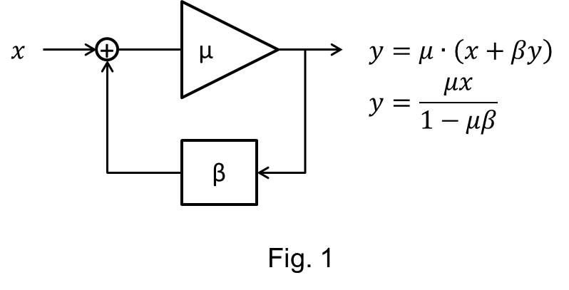
Depending on the application, a feedback system can be quite complex. Such systems are often described by nonlinear vector differential equations. But for the sake of simplicity we’ll consider just the equilibrium, i.e. algebraic, equations of the scalar feedback system depicted in Fig. 1.
If it weren’t for that system’s lower, β branch, the system output y would be simply the product μx of an open-loop gain μ and the input x. But the β branch adds to the input x a feedback quantity βy—i.e., a quantity responsive to the output y—and the input-output relationship consequently becomes y = μ · (x + βy). Isolating y gives the following explicit equation for the output:
where y' ≡ μx is what the output would have been without feedback, and the loop gain f ≡ μβ is what Lord Monckton sometimes calls the “feedback factor” or “feedback fraction.”
We will now see what his ambiguous, convoluted language tends to hide: that the “correction” he made in the American Thinker piece and those he’s made elsewhere are dictated by an implicit assumption: that y is linearly proportional to y', i.e., that f is a constant independent of x and y.
The Numbers
If we credit the numbers Lord Monckton used in his American Thinker piece, the pre-industrial (e.g., year-1850) equilibrium global-average surface temperature E was 57°F, which is 287 K on the absolute, Kelvin scale. (The equilibrium temperature associated with given conditions of, say, carbon-dioxide concentration can roughly be described as the temperature on which the earth would settle after those conditions had prevailed unchanged for a long enough time.)
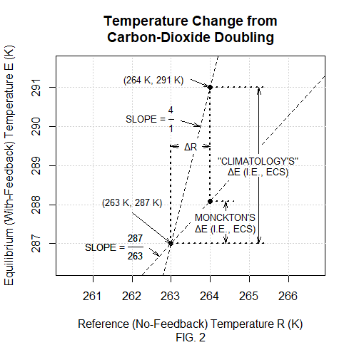
Also according to that piece, 24 K of that 287 K results from feedback; sunshine and other “direct” causes like carbon dioxide and other non-condensing greenhouse gases would have resulted in only 263 K without, e.g., the resultant temperature-dependent evaporation of water. That makes 263 K the pre-industrial value of what Lord Monckton called the “reference signal” R: it’s the without-feedback temperature for which, as the coordinates of Fig. 2’s bottom dot indicate, the with-feedback temperature E has its pre-industrial value 287 K.
(We digress at this point to acknowledge that we’re averting our eyes from the questionable nature of various assumptions such as that anyone actually knows what the temperature would be without feedback and that there’s a one-to-one relationship between values with and without feedback—and, indeed, that there really is such a thing as an equilibrium global-average surface temperature in a nonlinear, chaotic climate system. We focus instead on those admittedly questionable assumptions’ mathematical implications.)
The common horizontal distance ΔR between the bottom dot and the other two dots is the 1.0 K used by the American Thinker piece as the “direct warming” from doubling carbon dioxide, i.e., as the temperature increase that carbon-dioxide doubling would cause if there were no feedback. The ΔE = 4.0 K vertical distance between the top and bottom dots is the ECS value given by that article as a model exaggeration.
Linear Proportionality
Fig. 2’s “slope = 287/263” diagonal line represents the linear E(R) function that the “grave error” theory’s implied proportionality requirement dictates. So the middle dot represents the resultant “correction”: Lord Monckton multiplies the direct warming ΔR by the bottom-dot value of that function’s average slope E/R to extrapolate a low ECS value: ΔE/ΔR must equal E/R, so ΔE must be 1.1 K.
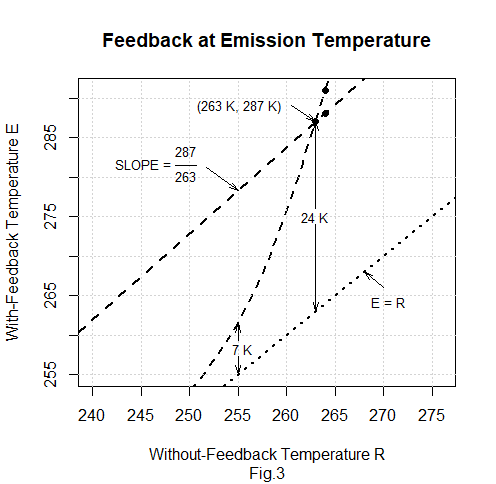
As Fig. 3 illustrates, the American Thinker piece’s statement that “nearly all feedback response in 1850 was a response not to preindustrial greenhouse gases but to the sunshine” is merely a corollary of the “grave error” theory’s linearity requirement. The 24 K vertical distance at R = 263 K between the linear-E(R), slope = 287/263 line and the zero-feedback, E = R line is the “corrected” E(R) function’s feedback response. According to that function, the feedback response doesn’t change much between 263 K and the “sunshine-only emission temperature of 255 K” in which subtracting the non-condensing greenhouse gases’ 8 K contribution from 263 K results. Specifically, the feedback response at R = 255 K is only about 1K less than the 24 K at R = 263 K.
Nonlinear Feedback
That would all make perfect sense—and feedback theory would therefore require that ECS be low—if such linear proportionality were indeed required by “the mathematics of feedback in all dynamical systems including the climate.” And such mathematics, according to Lord Monckton’s statement at time stamp 39:18 in the video of the March 27, 2017, speech in which he introduced the “grave error” theory to the Heartland Institute, “comes from electronic circuitry.” But by reference to an electronic feedback circuit we’ll show that nothing in feedback theory rules out a high-ECS, and therefore nonlinear, E(R) function such as the one that’s represented by Fig. 3’s dashed curve and exhibits only 7 K of feedback “to the sunshine.”
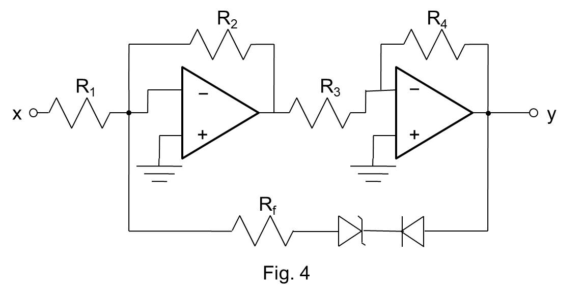
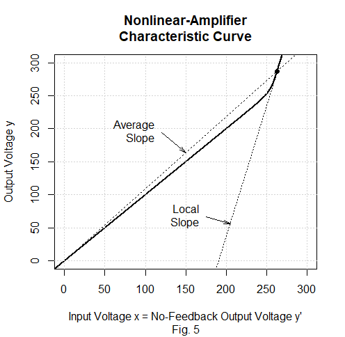
Fig. 4 depicts that circuit, whose characteristic curve numerically equals Fig. 3’s nonlinear E(R) function. (Readers unfamiliar with electronics are invited to skip the next three paragraphs’ circuit description, which isn’t critical to the remainder of the discussion.)
Corresponding to Fig. 1’s β block is Fig. 4’s feedback network, which consists of the lower-path series connection of two diodes and a resistor. To make the input x analogous to the without-feedback temperature R, the two operational amplifiers and the remaining four (equal-value) resistors comprise a unity-gain amplifier: they correspond to Fig. 1’s μ block, but with μ = 1.
Since the feedback path’s two diodes are connected in opposition, that path conducts negligible current, and thus provides negligible feedback, until the zener diode’s reverse voltage exceeds its zener voltage. We’re treating the zener voltage as being roughly 255 volts in order to make voltages numerically match the temperatures of Figs. 2 and 3, although we’d employ more-typical component values and scale voltages down by, say, a factor of ten if we were actually building the circuit.
Once the zener voltage is exceeded, the diodes’ incremental, “small-signal” resistance becomes small in comparison with the feedback-network resistor’s resistance, which is about a third again the other resistors’. As a consequence, feedback then becomes significant, and the circuit’s small-signal closed-circuit gain increases from barely more than 1 to about 4.
Again, there’s no need to understand all of the foregoing circuit description. What’s important is just that because the circuit’s upper branch is a unity-gain amplifier the input x is the same as the value y' the output would assume if there were no feedback. So the input x = y' is analogous to Lord Monckton’s reference (i.e., no-feedback) temperature R, while the actual output y is analogous to his equilibrium (with-feedback) temperature E.
Fig. 5 shows that the upper end of the circuit’s characteristic curve numerically equals Fig. 3’s nonlinear, high-ECS E(R) function. That function exhibits a high ECS value because, as the dotted lines indicate, its local slope at the pre-industrial state’s temperatures is about 3.7 times its average slope: feedback math doesn’t necessarily impose the linear-proportionality requirement that the logic of Lord Monckton’s “grave error” theory does.
“Suddenly Wake Up”
He nonetheless attempts to justify that requirement:
Climatologists universally but erroneously assume that all of the 25 K feedback response to date must be feedback response to the 8.5 K direct warming by natural and anthropogenic greenhouse gases.
In logic, climatologists’ position cannot be correct. For the feedback processes that subsist at any given moment in a dynamical system such as the climate are inanimate. They have no freedom to decide that they will not respond at all to the first 29/30 of the 263.5 K total reference temperature in 2020, but that they will respond only, and suddenly, and very vigorously, to the final 1/30. Where is the sense in that?
Therefore, at any specified moment, such as the present, the feedback processes subsisting in the dynamical system of interest, the climate, must perforce respond equally to each degree of the 263.5 K total reference temperature.
He had expressed a similar view some years earlier:
The central point, which swamps any mere considerations of nonlinearity, is that a temperature feedback response respondes [sic] to a temperature, and it has no way of deciding that it will not respond to emission temperature of 255 K but will suddenly wake up and respond only to the next 8 K of temperature.
That reasoning betrays a peculiar misunderstanding of how the physical world works. He might as well have said that our circuit’s zener diode has no way of deciding that it won’t conduct current below its zener voltage but will “suddenly wake up and” conduct current when its zener voltage is exceeded.
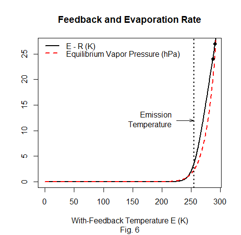
In that connection compare Fig. 6’s solid black and dashed red curves. The former plots against E the feedback response E – R of our hypothetical high-ECS E(R) function, while the latter plots against E what’s widely accepted as the resultant rate of water evaporation in terms of the water-vapor partial pressure that would make condensation cancel out evaporation.
Both quantities are nearly zero until the temperature approaches the “sunshine-only emission temperature of 255 K.” Since water’s temperature dependence is what’s primarily considered responsible for the climate’s temperature feedback, it’s entirely plausible that temperature feedback would “suddenly wake up” in that range.
Now, despite evaporation’s high sensitivity to temperature there are good reasons for believing that on the contrary the feedback response is not as pronounced as Fig. 6 indicates—and that ECS is accordingly as low as Lord Monckton contends. But that doesn’t mean that high ECS estimates resulted from climate modelers’ failure to take the sun into account. Modelers more likely did take it into account in calculating evaporation rates, which as we’ve just seen actually do “suddenly wake up.” High ECS estimates probably just resulted from bad guesses modelers made about those evaporation rates’ implications.
Indeed, it’s hard to imagine how modelers could have managed to leave the sun out of feedback calculations. The models “tune” their “parameterizations” to make results match recent decades’ observed temperatures, and they couldn’t arrive at those temperatures without taking the sun into account; without sunshine the earth would be an ice ball. Since the feedback in those models results mostly from evaporation, which in turn depends on temperature values thus based on sunshine, how could the models possibly manage to calculate feedback without taking the sun into account?
Apples to Oranges
As we’ve seen, and as critics immediately recognized when the “grave error” theory debuted on the Watts Up With That site, Lord Monckton’s arguments logically require linear proportionality; feedback math would rule out high ECS values only if it required that feedback systems be at least substantially linear. However, although Lord Monckton has long conceded as he must that the climate system is nonlinear, he argues that it can’t be nonlinear enough to matter.
His argument for that proposition has varied. At the time of that March 2018 debut post it took the form of some barely intelligible word salad that ultimately begged the question. He’s since favored versions that are so convoluted as largely to mask what they really are: apples-to-oranges comparisons. An elaborate example, which he delivered in July 2019 at the Heartland Institute's Thirteenth International Conference on Climate Change, can be viewed in the six-minute segment that begins at time stamp 21:45 of his speech’s video.
He has since refined that argument, eventually boiling it down to the following one-sentence version taken from his July 8, 2021, blog post:
[G]iven that RCS is little more than 1 K, it is scarcely credible that ECS will fall on the currently-implicit interval 4 [2, 6] K, for that would imply, per impossibile, that the doubled-CO2 unit feedback response 3 [1, 5] would exceed the industrial-era unit feedback response 1.1 – 1 = 0.1 by a factor 30 [10, 50].
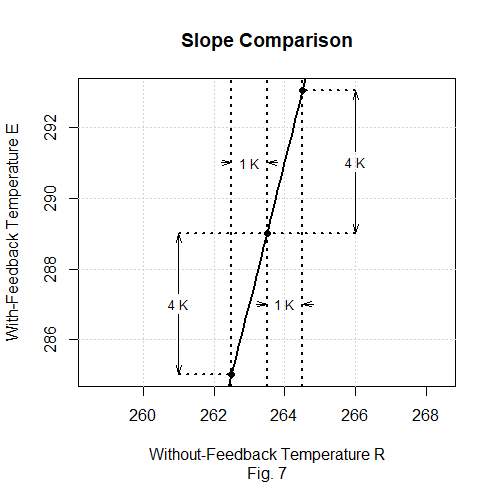
To unpack that argument and appreciate its apples-to-oranges nature, consider the segment of our hypothetical E(R) function that Fig. 7 displays.
That plot’s middle dot represents the “industrial era,” to which Lord Monckton had assigned the without-feedback temperature R = 263.5 earlier in the post. Increasing R by his 1 K value of “RCS,” as he calls the change ΔR that doubling carbon dioxide would cause without feedback, raises the with-feedback temperature E by about 4 K because E(R)’s slope is about 4. Nearly the same change in E occurred in the previous 1 K change, from 262.5 K to 263.5 K, because the difference between the slope’s averages over the two intervals is slight; those averages are 3.98 and 4.04.
Those averages’ ratio, 1.015, would be the apples-to-apples comparison; we’ve compared equal-width intervals. What Lord Monckton does instead is compare the 1 K interval between 263.5 K and 264.5 K with the 263.5 K interval between absolute zero and 263.5 K. With rounding, the slope’s averages over those intervals are respectively 4.0 and 1.1, but Lord Monckton prefers to subtract 1.0 from those averages to get 3.0 and 0.1 as his values of what he respectively calls the “doubled-CO2 unit feedback response” and the “industrial-era unit feedback response.”
Those values are his basis for contending that an ECS of 4 is “scarcely credible” because it “would imply, per impossibile, that the doubled-CO2 unit feedback response 3 [1, 5] would exceed the industrial-era unit feedback response 1.1 – 1 = 0.1 by a factor 30.” His reason for calling an ECS value of 4 K “scarcely credible,” in other words, is that he can subject the thereby-implied 1.5% slope change to mathematical operations he’s concocted and get 30 as his result.
Although Lord Monckton says he’s “trained in classical logic,” such a non sequitur is typical of his reasoning: his premise, which in this case is that the ratio of vastly different intervals’ unit feedback responses is 30, has no logical connection to the conclusion he draws from it, i.e., that ECS is low.
Conclusion
To be clear, there are indeed good reasons for believing that ECS is low, and some of those reasons even make occasional appearances in the thousands of words Lord Monckton has written about the purported “grave error.” But the continued acceptance in some circles of the fantastic proposition that modelers’ forgetting sunshine is the reason for high ECS estimates is a tribute to how vague and impressionistic Lord Monckton’s writing is.
Readers seeking a flavor of that writing could do worse than consider the post in which Lord Monckton responded to critics and ended the post with what he triumphantly called “the end of the global warming scam in a single slide.” Now, when that slide’s numbers are actually graphed they’re seen to be what even a high-school analytic-geometry student could recognize as bad extrapolation. But to a superficial reading—which, let’s face it, is all most of us usually have time for—his post can seem to provide cogent responses.
Closer analysis would show instead that it’s self-contradictory and does little more than assert implications of his theory’s implied linearity requirement and make apples-to-oranges comparisons. But in view of the prominence that the Heartland Institute, Watts Up With That, and now American Thinker have given the “grave error” theory over the years such closer analysis seems thin on the ground.
Apparently if your language is obscure enough you really can fool some of the people all of the time.

